Understanding Primary Secondary Pumping Part 2: Mixing Temperatures (and Flows!) in a Hydronic System
/By Chris Edmondson
What happens in a pipe when water of two different temperatures (and perhaps different flow rates) merge?
There’s a pretty straightforward formula that tells you exactly what the resultant water temperature will be. In this blog, we’ll go over that calculation, as well as take a closer look at how blended temperatures and flows impact the performance of primary secondary systems. The laws of physics cannot be denied in chilled (or hot water) system design, therefore it is important to have a solid understanding of these fundamental principles in order to make good design or troubleshooting decisions.
So let’s take a look at blended temperatures in a hydronic system. Figure 1 shows a very simple example of a piping tee with blended temperatures and flows. The calculation below the diagram demonstrates exactly how we determine what the temperature of the water on the right side of the tee will be after the blending of the 100 GPM at 40°F and 50 GPM at 55°F. We simply multiple the flow and temperature of the two pipes about to merge flow, add those values together, and divide by the resulting flow to get the temperature of the blended water, which, in our example turns out to be 45°F.

Figure 1
Now let’s apply this to an actual primary/secondary hydronic system.
Figure 2 shows a system that is not balanced (meaning that the flow in the secondary loop is not the same as the primary loop.) As we discussed in Part 1 of this series, this scenario will result in reverse flow in the common (green) pipe. In our Figure 2 example, we would have precisely 60 GPM of reverse flow. Knowing what we know about blended temperatures and flow, how will this impact the supply water temperature to the secondary circuit in a hydronic system?
Keep in mind that in this example our cooling coil has been designed for a 45°F supply temperature and a Delta T (∆T) of 10 degrees. This is pretty typical, since these are the approximate temperatures required in a hydronic cooling system to achieve proper dehumidification of the air. That’s our target – but what if for some reason we start overflowing the secondary circuit with 180 GPM?

Figure 2
If we zero in on what is happening in the common pipe and apply the formula we used above, we notice that all of the sudden instead of a 45°F supply temperature to the coil, we now have approximately 48°F going to the coil:
(120 GPM x 45°F) + (60 GPM x 55°F) = 180 GPM x T
T= 48.333
That’s a problem. A 48°F supply temperature is not low enough to achieve proper dehumidification in the coil. The best way to fix this is to install a balancing valve or circuit setter in the secondary loop to reduce the flow back down to 120 GPM. Then our flows are balanced and our target secondary supply temperature of 45°F and design 10 ∆T is maintained. Also, our chillers will be satisfied because they are getting the 55°F return water temperature for which they were designed.
Unfortunately, balancing the secondary loop with the primary loop is not always the first solution that springs to mind. Some might decide to increase the flow in the primary loop since that would eliminate the reverse flow in the common pipe and stop the blending of warm return water with cold supply water. (Figure 3)

Figure 3
This solution works for meeting our cooling and dehumidification requirements, but it creates a problem with our chillers. Why? Because now we have 52°F going back to the chillers when we should have 55°F. Under these circumstances the chiller will not load properly and you will never get the designed tonnage out of the chiller plant!
Making Different Flows Work
This doesn’t mean that flows in the primary and secondary loop have to be the same. Properly designed, you can have greater flow in the secondary loop and still bring back 45°F water back to your secondary circuit and 55 °F to the chillers. It’s all in the math.
Consider the example below (Figure 4) and the following formula:
BTUH
GPM = 500 x ∆T
In our example, our cooling coil is designed to remove 750,000 BTUHs from the secondary supply water. (Note that we have 40 °F in the primary supply, 45 °F in the secondary supply and a ∆T to 10 degrees at our coiling coil.)

Figure 4
Using the formula GPM = BTUH / 500 X ∆T,we can determine that we have the following flow in our primary and secondary loop:
750,000
500 x 10 = 150 GPM in secondary loop
750,000
500 x 15 = 100 GPM in the primary loop
So, as you can see in Figure 4, all is well with our supply temperatures and all is well with the temperature going to our chiller. Yes, we have 50 GPM of reverse flow in the common pipe, but because we’ve lowered our primary supply temperature to 40 degrees, we are still able to deliver 45 degrees to our secondary circuit. Again, it’s all in the math:
(100 GPM x 40 °F) + (50 GPM x 55 °F) = 150 x T
thus,
T = 45°F